Closing — The Three-Step Summary

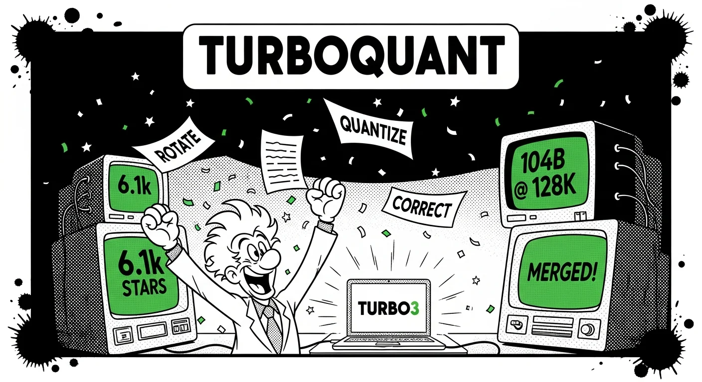
We’ve covered a lot of ground. Let’s bring it back to the essentials.

The Problem in One Sentence

Every token you generate stores a Key and Value vector at every layer of the model. At scale – millions of users, 128K context windows, 70B parameters – this fills your GPU faster than the model weights do. FP8 KV cache gives a free 2× from hardware; TurboQuant gives the next 2-3× from mathematics.

The Insight in Three Steps

Step 1 — Rotate

Apply a random rotation matrix (in practice: Walsh-Hadamard Transform + random signs) to each KV vector. This redistributes whatever “spiky” structure the raw vectors had into a smooth, near-Gaussian distribution. The rotation preserves inner products perfectly — it’s a change of coordinates, not a change of information. Fuse this into the attention write kernel to keep overhead negligible on GPU.

Step 2 — Quantize

Apply Lloyd-Max scalar quantization to the rotated, near-Gaussian vector. Because the distribution is now Gaussian, the codebook is optimal for that distribution. Theory guarantees you’re within 2.72× of the information-theoretic limit — closer than any other practical online algorithm. Remember that codebook centroids scale with $1/\sqrt{d}$ for your specific head dimension.

Step 3 — Correct (when needed)

If you’re below 3 bits, add a 1-bit QJL sketch of the residual to eliminate the systematic bias that the MSE quantizer introduces. Above 3 bits, the bias is small enough (~3%) that softmax tolerates it, and the correction step’s variance costs more than it saves.

b ≤ 2:   Rotate → Quantize (b-1 bits) → QJL residual
b ≥ 3:   Rotate → Quantize (b bits)

The Results in Three Numbers

• 3.5 bits — the bit-width at which TurboQuant achieves zero measurable quality loss on LongBench across six task types
• 4.6× — the compression ratio at 3.5 bits (vs FP16; 2.3× additional over FP8 KV)
• 0.997 — TurboQuant’s Needle-in-a-Haystack recall at 128K context, identical to the uncompressed baseline

Who Should Care

If you run inference today: Start with FP8 KV cache — it ships in vLLM, TGI, and TensorRT-LLM, requires zero configuration changes, and gives 2× KV compression for free on H100/H200/B200. If you need more than 2×, add TurboQuant via the turboquant+ library (CUDA, ROCm, Metal, CPU). The practical recipe: turbo4 for quality-first, turbo3 for maximum throughput. Keys at 4 bits, Values at 2 bits, boundary layers protected at higher precision.

If you’re building serving infrastructure: The W4A8KV4 stack is the current production sweet spot for H100:

W4  (4-bit weights):     GPTQ or AWQ — reduces weight memory 4×
A8  (FP8 activations):   hardware-native on H100+ — ~1.8× compute throughput
KV8 (FP8 KV cache):      hardware-native, 2× KV compression, deploy first
KV4 (TurboQuant):        software, additional 2× over FP8, deploy when KV is the limit

Stack effect on 70B @ 128K context:
  Weights 140 GB → 35 GB
  KV cache 16 GB/user → 4 GB/user
  ~4× more concurrent users per GPU
  ~2× faster decode throughput

PagedAttention manages allocation; FlashAttention handles prefill bandwidth; TurboQuant handles decode KV bandwidth. In disaggregated serving, TurboQuant also compresses inter-node KV transfers — most valuable on InfiniBand-connected clusters, less so on NVSwitch rack-scale systems.

If you’re evaluating SSM/Mamba-style alternatives: SSMs trade long-range retrieval fidelity for the elimination of KV cache growth. For workloads where exact retrieval matters — agents, RAG, legal/medical documents — attention with TurboQuant compression remains the more reliable architecture. For throughput-first workloads where fine-grained retrieval does not matter, SSMs are a legitimate alternative. The choice is workload-dependent.

If you’re training new models: Consider MLA (DeepSeek’s architectural approach) during pretraining. MLA achieves sub-0.1× KV cache compression without any inference-time quantization, at the cost of a different training-time architecture. TurboQuant and MLA address the same problem at different stages: TurboQuant is the best compression for models that exist today; MLA is the architectural choice for models being trained tomorrow.

If you’re on Blackwell: NVFP4 hardware-native 4-bit support creates a future path to zero-overhead KV4 compression. TurboQuant currently uses INT4 codebook indices; mapping these to Blackwell’s E2M1 FP4 format is an open engineering question. When solved, turbo4 on B200 could run with the same hardware efficiency as FP8 on H100. Watch for TensorRT-LLM kernel integration as the signal that this path is production-ready.

The Competitive Landscape — Why the Timing Matters

TurboQuant was published at ICLR 2026 with the paper and blog post but no official code. The community filled that gap within weeks.

The reason the timing matters: Google has implementation advantages that no one else does.

Google can integrate TurboQuant directly into XLA and TPU firmware — fused into the attention kernel at the hardware level, running on custom silicon they manufacture. The algorithm’s rotation and quantization steps are small, regular computations that map well to TPU systolic arrays. An XLA-native implementation could achieve lower latency and higher throughput than any GPU-based implementation because the quantization overhead essentially disappears into the prefill and decode pipelines.

The community implementations on CUDA, ROCm, and Metal are genuine and production-ready. But they are running on hardware designed for different workloads. Google’s advantage is the ability to co-design the algorithm’s execution with the hardware it runs on.

Community (CUDA/ROCm/Metal):    Algorithm + hardware, separately optimized
Google (TPU + XLA + firmware):  Algorithm + hardware, co-designed
                                 Near-zero quantization overhead
                                 Already have the serving infrastructure at scale

The algorithm is public. The math is the same for everyone. The race now is implementation quality, hardware efficiency, and integration depth — and that race has already started.

The One-Slide Version

Problem:   KV cache grows without bound. At 128K context, it exceeds the model weights.
           FP8 KV gives 2× free. TurboQuant gives the next 2-3×.

Algorithm: Rotate (WHT + signs) → near-Gaussian distribution.
           Quantize (Lloyd-Max, codebook scaled by 1/√d) → within 2.72× of optimum.
           At 3+ bits, skip the QJL bias correction.

Result:    3.5 bits per coordinate. Zero quality loss. 4.6× compression over FP16.
           104B model. 128K context. One MacBook.

Production: W4A8KV4. FP8 first. TurboQuant for the second 2×. Fuse into the kernel.

What's next: TensorRT-LLM kernel integration. Blackwell FP4 alignment.
             Disaggregated KV transfer compression.
             And Google racing to productionize this on TPUs.