The Random Rotation — Making Any Vector Predictable
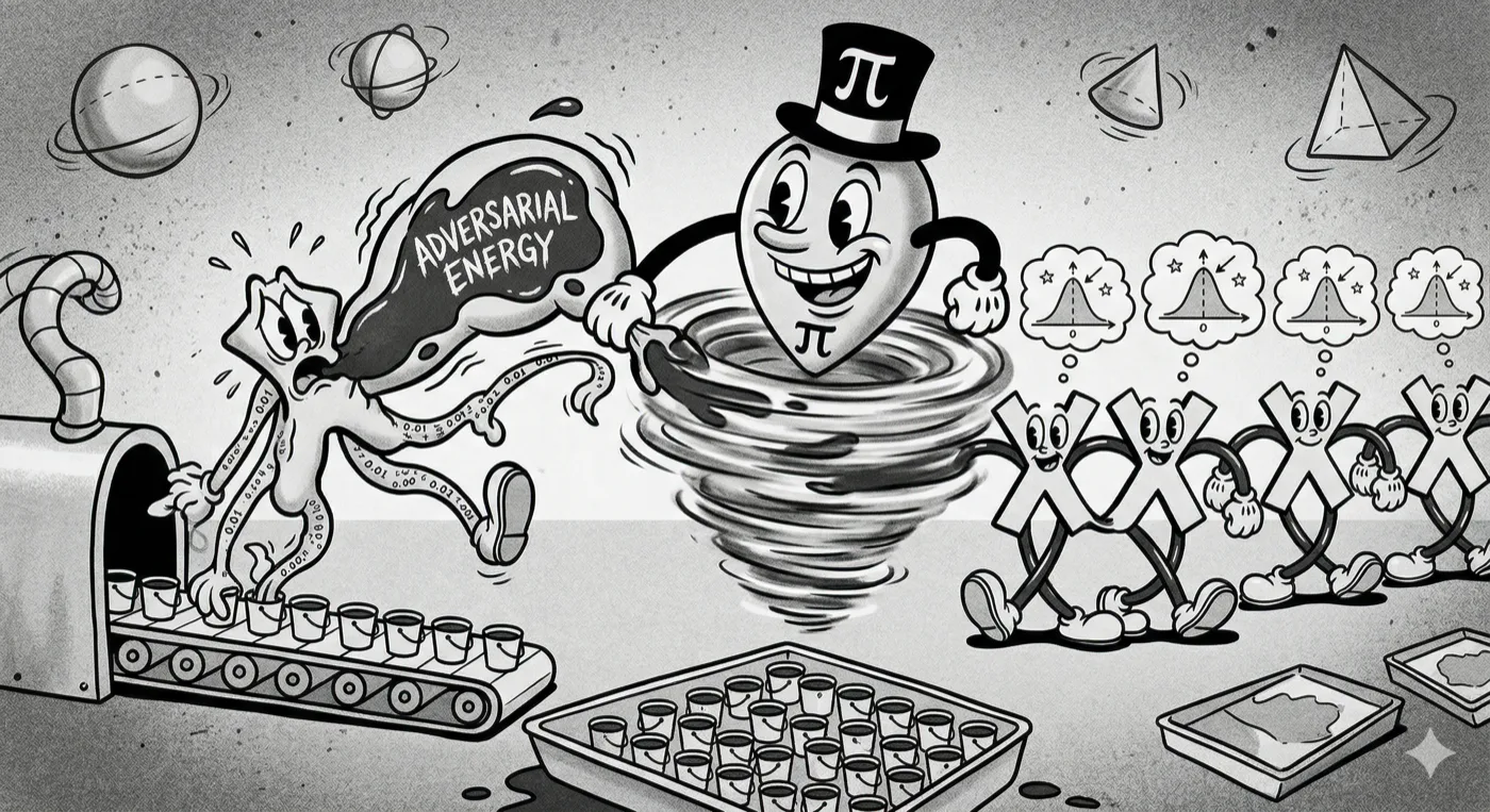
We have two problems from the last two sections. We need to know the distribution of our data to design an optimal codebook – but KV cache data is unpredictable. And we need coordinates to be independent for scalar quantization to be optimal – but real vectors have correlated coordinates.
TurboQuant solves both problems with a single operation: multiply the vector by a random rotation matrix.
What Is a Rotation Matrix?
A rotation matrix is a square matrix $\Pi$ that, when multiplied with a vector, rotates the vector without changing its length.
Properties of a rotation matrix Pi:
  1. ||Pi . x|| = ||x||         <- preserves vector length
  2. <Pi.x, Pi.y> = <x, y>     <- preserves inner products (!)
  3. Pi . Pi^T = I              <- its inverse is its transpose (orthogonal)
Property 2 is extremely important: rotation preserves all inner products. If we rotate all vectors by the same rotation matrix, every dot product between every pair of vectors is exactly the same as before. The geometry is completely preserved.
In 2D:
$$\Pi = \begin{bmatrix} \cos\theta & -\sin\theta \ \sin\theta & \cos\theta \end{bmatrix}$$
In $d$ dimensions, you generate a random rotation matrix by:
- Generate a $d \times d$ matrix with i.i.d. entries from $N(0, 1)$
- Apply QR decomposition
- The Q matrix is your random rotation matrix
Rotation changes the coordinates of a vector without changing the vector itself. It’s a change of basis, not a change of information.
The 2D Example
Consider a unit vector that’s “adversarial” – all its energy concentrated in one coordinate:
Original vector: x = (1.0, 0.0)

  y-axis
    |
    |
    |
    *-----------> x-axis
  (0,0)         (1,0)
After a 45° rotation:
Rotated vector: x' = (0.707, 0.707)

  y-axis
    |       /
    |     /
    |   / x'
    | /
    *-----------> x-axis
  (0,0)
The energy is now spread equally across both coordinates. Quantizing this rotated vector is much easier – neither coordinate dominates the error.
A random rotation in d dimensions spreads the energy of any input vector nearly uniformly across all d coordinates.
Why Randomness Makes the Distribution Predictable
This seems paradoxical: adding randomness makes things more predictable? Here’s the intuition:
Before rotation: The distribution of coordinates depends on the input vector. For a vector pointing mostly in direction 1, coordinate 1 is large and coordinate 2 is small. The distribution is input-dependent – unpredictable.
After a random rotation: By the concentration of measure on the sphere (specifically, the Haar-measure property of random orthogonal matrices), each coordinate of the rotated vector is approximately:
$$y_i = [\Pi x]_i \sim N!\left(0, \frac{|x|^2}{d}\right)$$
The distribution of each coordinate after a random rotation is Gaussian, with variance determined only by the vector’s length – not by its direction. Since we normalize vectors to unit length before quantization, the distribution is always $N(0, 1/d)$, regardless of input.
After a random rotation, every vector’s coordinates follow the same distribution. The codebook can be precomputed once from this known Gaussian distribution and works for all inputs forever.
This solves Problem 1 from Section 5 (needing to know the distribution). It also makes the coordinates independent (approximately), solving Problem 2 (correlated coordinates).
How Well Does Gaussianization Work? The Role of Dimension d
The Johnson-Lindenstrauss approximation is not exact — it is asymptotically correct as dimension $d$ increases. A larger $d$ means more random projections contribute to each rotated coordinate, and the central limit theorem convergence is tighter.
This has a practical implication: the quality of Gaussianization after WHT depends on the head dimension of the model you’re compressing.
d = 1536  (OpenAI embedding models):
  → Very good Gaussianization. Close to the theoretical guarantee.
  → Paper's primary validation target.

d = 128   (Llama 3, Mistral, Gemma, Qwen):
  → Good Gaussianization. Some residual non-Gaussianity remains.
  → Community kurtosis measurements: 900 → ~2.9 after WHT (Gaussian target: 3.0)
  → Confirmed to work well empirically across 30+ hardware configs.

d = 64    (older models, some efficient variants):
  → Weaker Gaussianization. The theoretical bound is looser.
  → More aggressive compression (turbo2) may show quality degradation faster.
  → Validate empirically before deploying turbo3 or below.
The community results (Section 15) confirm the algorithm works at d=128 — the validation came from empirical testing, not the paper’s theoretical guarantee. If you’re deploying on a model with d=64, run your own perplexity tests before assuming the standard bit-width recommendations hold.
The Practical Implementation: Walsh-Hadamard Transform
The theory uses a random Gaussian rotation matrix $\Pi$ of size $d \times d$. For $d = 128$, that’s 16,384 floating point numbers to store and multiply. For real-time KV cache compression – handling millions of tokens per second – this is too slow.
In practice, every implementation uses the Walsh-Hadamard Transform (WHT) instead.
What Is the WHT?
The WHT is a specific structured rotation matrix whose entries are all $\pm 1 / \sqrt{d}$. In 4D:
H_4 =  1/2 × [ 1   1   1   1 ]
              [ 1  -1   1  -1 ]
              [ 1   1  -1  -1 ]
              [ 1  -1  -1   1 ]
The matrix is built recursively: $H_{2d} = \frac{1}{\sqrt{2}} \begin{bmatrix} H_d & H_d \ H_d & -H_d \end{bmatrix}$, so it’s always a power of 2 in size.
Why WHT Instead of Gaussian Rotation?
Three reasons:
Speed: The naive matrix multiply for a $d$-dimensional rotation costs $O(d^2)$ operations. The WHT can be computed in $O(d \log d)$ using a fast butterfly algorithm – the same structure as the FFT. For $d = 128$, that’s 128² = 16,384 vs 128 × 7 ≈ 896 multiply-adds. About 18× fewer operations.
Memory: The Gaussian rotation matrix requires storing $d^2$ floats ($128^2 = 16$K parameters). The WHT needs no stored matrix at all – the structure is implicit in the algorithm.
Randomization: WHT alone is a fixed, deterministic rotation (not random). To introduce randomness, you combine it with a random diagonal sign matrix $D$ applied before the transform: the full operation is $x’ = H \cdot D \cdot x$, where $D_{ii} \in {+1, -1}$ uniformly at random. This combined operation – sometimes written HD or RHDH – has the same statistical properties as a full random rotation at a fraction of the cost.
Practical rotation step:

  D = random diagonal matrix with ±1 on diagonal (one per inference session)
  H = Walsh-Hadamard matrix (no storage needed, computed on the fly)

  y = H(D · x)    // O(d log d) time, O(d) extra memory for D
The turboquant+ community library and all major llama.cpp implementations use this HD variant.
GPU Implementation Note
On CPU (AVX-512) and Apple Silicon (AMX), WHT’s butterfly pattern maps efficiently to SIMD units. On CUDA, the stride-2 butterfly access pattern is less cache-friendly for GPU warps, which prefer coalesced 128-byte reads. The rotation step is negligible overhead when fused inside the attention kernel — doing the WHT while K/V data is already in registers, before the quantize-and-write step. Implemented as a standalone pre-processing pass over HBM, the overhead is measurable. Production CUDA implementations should fuse the rotation into the attention write path.
The llama.cpp benchmarks showing “speed parity with q8_0” are measured on CPU/Metal. These numbers are representative for that runtime; GPU implementations require kernel fusion to achieve comparable overhead.
The theoretical guarantees hold for both Gaussian and WHT rotations. WHT + random signs satisfies the orthogonality requirement. You get identical compression quality at 18× lower computational cost — provided the rotation is fused into the kernel on GPU.
On RoPE models: Section 3 flagged that modern LLMs (Llama, Mistral, Qwen, Gemma) apply RoPE positional encoding to the Query and Key vectors before they are written to the KV cache. TurboQuant therefore compresses RoPE-rotated Keys. RoPE rotates pairs of dimensions by angles proportional to position — it does not create large outliers or break the Gaussian approximation in any systematic way that the WHT cannot handle. Empirically, the community has confirmed TurboQuant works correctly on all tested RoPE models at d=128 (Section 15). The open question is whether very long-range RoPE extensions (e.g., Llama 3.1’s 8M-context variant, which uses frequency scaling) create distributional shifts that affect WHT Gaussianization — this has not been systematically tested.