Scalar Quantization 101
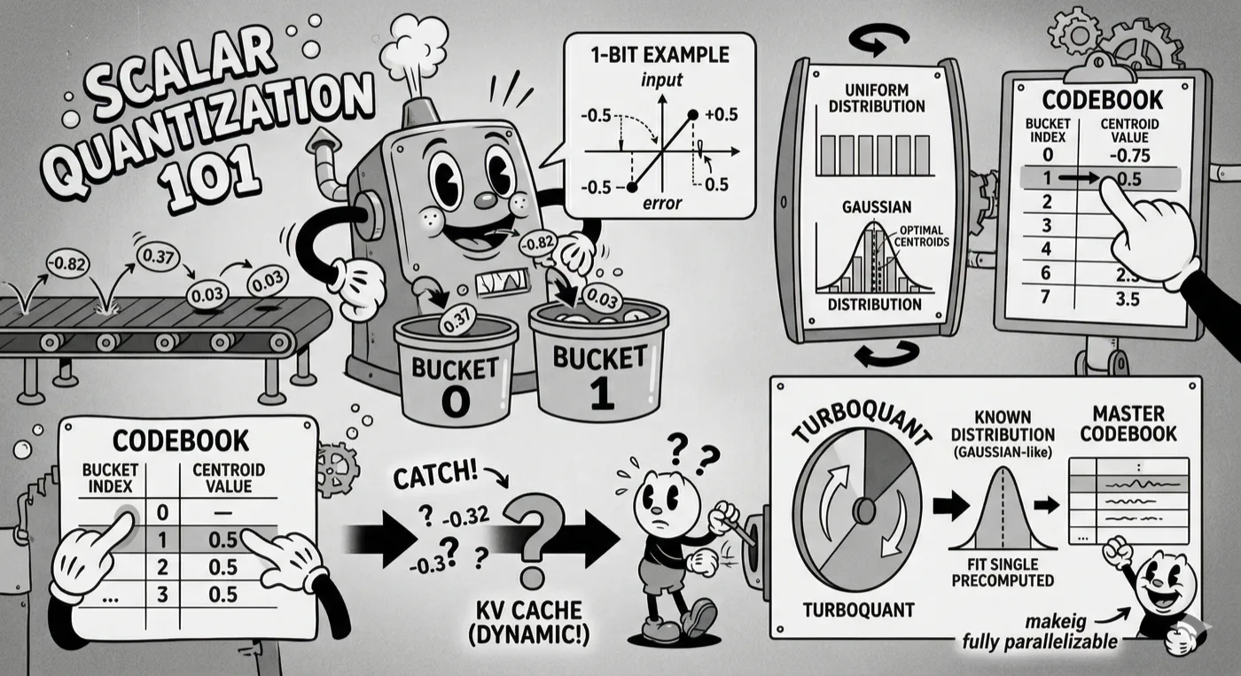
Before we get to TurboQuant, we need to understand the building block it uses: scalar quantization. This is the foundation. If you get this, TurboQuant will feel almost obvious.
Scalar quantization is the simplest form of compression: take a single real number, and replace it with the nearest value from a small, fixed set of allowed values.
1-Bit Quantization: The Simplest Case
You have a number that can be anything between -1 and 1. You’re allowed to store exactly 1 bit. That gives you $2^1 = 2$ possible stored values.
You need to choose:
- Two representative values (centroids): $c_1$ and $c_2$
- A boundary between them: any input below the boundary maps to $c_1$, above maps to $c_2$
The most obvious choice:
Boundary: 0
Centroid 1: -0.5    (represents all negative values)
Centroid 2: +0.5    (represents all positive values)

    -----------------+------------------
    -1     -0.5      0      0.5      1
           c1     boundary    c2

Input:  0.37  -> positive -> store bit "1" -> reconstruct as  0.5
Input: -0.82  -> negative -> store bit "0" -> reconstruct as -0.5
Input:  0.03  -> positive -> store bit "1" -> reconstruct as  0.5   <- big error!
That last one hurts. The value 0.03 is very close to zero, but it gets snapped to 0.5. The error is 0.47.
Is there a better choice of centroids? It depends on the distribution of your data.
Why Distribution Matters
Scenario A: Uniform Distribution
Values are equally likely to be anywhere between -1 and 1. For uniform data, equal-width buckets are actually optimal.
Scenario B: Gaussian Distribution
Most values cluster near zero, with few values near the extremes.
Probability
  |           /\
  |          /  \
  |         /    \
  |        /      \
  |      /          \
  |   /                \
  +--/--------------------\------
    -1        0            1
For Gaussian data, equal-width buckets are wasteful. Most values live near zero, so you want centroids closer to zero where the data is dense.
Scaling to Multiple Bits: The Lloyd-Max Quantizer
For $b$ bits, you have $2^b$ buckets and $2^b$ centroids. The Lloyd-Max quantizer finds the optimal placement by minimizing mean squared error for a given distribution. For a Gaussian with standard deviation $\sigma$, the 1-bit optimal centroids are at $\pm \sqrt{2/\pi} \cdot \sigma \approx \pm 0.7979\sigma$.
For TurboQuant specifically: after the rotation step (Section 8), each coordinate of a d-dimensional unit vector follows $N(0, 1/d)$, so $\sigma = 1/\sqrt{d}$. For d=128, $\sigma \approx 0.088$, and the actual codebook centroids are at approximately $\pm 0.7979 / \sqrt{128} \approx \pm 0.071$ — much smaller than the ±0.80 you’d use for σ=1. The Lloyd-Max tables must be computed for the specific σ of your head dimension d.
b=1 centroids (illustrative, σ=1):  [-0.80, +0.80]
b=2 centroids (illustrative, σ=1):  [-1.22, -0.40, +0.40, +1.22]
b=3 centroids (illustrative, σ=1):  [-1.75, -1.05, -0.50, -0.15, +0.15, +0.50, +1.05, +1.75]
b=4 centroids (illustrative, σ=1):  16 values, dense near zero, sparse at tails
Each time you add a bit, error drops by roughly 4x. This is the fundamental compression law: one more bit = one more bit of precision = 4x less distortion.
Quantization in Blocks — Why Block Size Matters
In practice, quantization is applied not to individual numbers in isolation but to blocks of numbers together. Each block gets its own scale factor that adapts to that block’s magnitude range.
Block quantization (block_size = 4, b = 2 bits):

  Raw values:    [0.41,  0.08, -0.33,  0.67]
  Block max:     0.67
  Normalized:    [0.61,  0.12, -0.49,  1.00]   <- scale to [-1, 1]
  Quantized:     [1,     0,    -1,      2  ]   <- 2-bit indices
  Scale stored:  0.67 (16-bit float)

  Effective bits per value:
    2 bits per value + 16-bit scale / block_size
    = 2 + 16/4 = 6 bits per value  ← worse than unquantized at small blocks!
This reveals why block size is a critical hyperparameter, not an implementation detail:
| Block size | Overhead (16-bit scale / block) | Effective bits at b=4 |
|---|---|---|
| 16 | 1.00 bit/val | 5.00 |
| 32 | 0.50 bit/val | 4.50 |
| 64 | 0.25 bit/val | 4.25 |
| 128 | 0.125 bit/val | 4.125 |
| 256 | 0.063 bit/val | 4.063 |
Larger block size → less overhead → better effective compression, but the scale factor covers more values, so extreme outliers within the block increase quantization error for all values in the block.
Smaller block size → more overhead → worse compression, but each block adapts more finely to local magnitude variations, preserving accuracy.
The turboquant+ community uses block_size = 128 by default — the same block size used by GGUF weight quantization and llama.cpp’s Q4_K format. This is not a coincidence: 128 elements maps well to SIMD vector widths on both AVX-512 CPUs and CUDA warp operations, and it gives the 5.12× compression figure cited for turbo3.
When you see compression ratios like “5.12×”, check the block size. The effective bit-width is
b + scale_bits/block_size, wherescale_bitsis 16 for FP16/BF16 scale storage (the turboquant+ default and llama.cpp GGUF formats) or 32 for FP32 scale storage. At the default 16-bit scale: block size 128 at 3 bits → 3.125 effective bits → 16/3.125 = 5.12× compression. Implementations using FP32 scale factors give 3.375 bits at block_size=128 — an 8% difference worth verifying for your deployment.
Error Types: Random Noise vs Systematic Bias
There are two fundamentally different ways a quantizer can be wrong:
Random noise — the reconstruction error is unpredictable but zero on average:
True value: 0.43
Reconstructed: 0.43 + noise   where noise is sometimes positive, sometimes negative
Average error: 0
Systematic bias — the reconstruction is consistently wrong in the same direction:
True value: 0.43
Reconstructed: 0.43 + 0.05   always slightly too high
Average error: +0.05 (never cancels out)
For compression tasks where you reconstruct the original data (images, audio), random noise is acceptable – it averages out. But for inner products in attention, systematic bias is more dangerous: it makes the model consistently over- or under-estimate the relevance of certain tokens.
The distinction between MSE (quantization accuracy) and bias (systematic error) is the core tension TurboQuant is designed to resolve. Sections 8-11 explain how it does this.
A Note on Integer vs Floating-Point Quantization Formats
TurboQuant uses integer codebook quantization: each value is stored as an integer index into a precomputed Lloyd-Max codebook, and dequantized by table lookup. The indices are 2-bit, 3-bit, or 4-bit integers — not floating-point numbers.
This is the same format used by GGUF weight quantization (Q4_0, Q4_K_M, Q8_0). Comparing TurboQuant against these formats by effective bit-width is apples-to-apples.
However, NVIDIA’s Blackwell architecture (B200, B100) introduces native NVFP4 support — a 4-bit floating-point format (E2M1: 2 exponent bits, 1 mantissa bit, 1 sign bit). NVFP4 tensor core instructions operate on this specific format; they do not natively accelerate arbitrary 4-bit integer indices. TurboQuant’s INT4 codebook indices and Blackwell’s FP4 tensor core format are different representations.
TurboQuant INT4:  index 0-15 into a Lloyd-Max lookup table  → table lookup dequant
NVFP4 (E2M1):    4-bit floating-point number (range 0-6, 8 steps)  → hardware-native

To use TurboQuant on Blackwell FP4 hardware paths:
  Option A: Keep TurboQuant INT4, use custom CUDA kernel (no FP4 acceleration)
  Option B: Map Lloyd-Max centroids to nearest FP4 values (approximation, needs validation)
This is an open engineering question for the community. It does not affect CPU, Metal, or current-generation CUDA implementations — it only matters if you want to exploit Blackwell’s native FP4 paths specifically.
Effective Bit-Widths in Practice
GGUF weight quantization (for reference):
  Q4_0:    4.500 bits/weight (block_size=32,  scale=16 bits)
  Q4_K_M:  4.125 bits/weight (block_size=256, scale=16 bits)
  Q8_0:    8.500 bits/weight

TurboQuant KV cache quantization (block_size=128):
  turbo2:  2.125 bits/val  → 7.5× compression vs fp16
  turbo3:  3.125 bits/val  → 5.1× compression vs fp16
  turbo4:  4.125 bits/val  → 3.9× compression vs fp16

Hardware-native KV compression (for comparison):
  FP8 KV:  8.0 bits/val   → 2× compression vs fp16 (zero overhead on H100+)
This is why turbo4 at “4.125 bits” beats q4_0 at “4.500 bits” in quality: it achieves lower effective bit-width while using a superior quantization strategy (rotation-based Gaussianization vs direct uniform quantization). And it’s why FP8 KV is the right starting point before considering TurboQuant — you get 2× for free, and TurboQuant gets you the next 2× at the cost of software complexity.