Why Compressing the KV Cache Is Hard
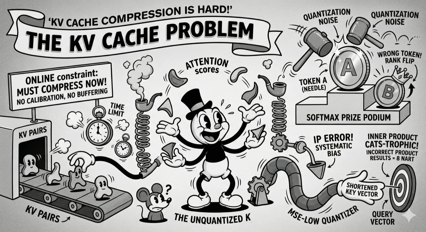
Before asking “can we compress the KV cache?”, it helps to ask “how far can we get for free?”
The easy step — FP8 — is already solved. H100, H200, and B200 all have hardware-native FP8 tensor cores. Storing the KV cache in FP8 instead of FP16 gives 2× compression with zero algorithmic overhead, zero rotation, zero codebook lookup. It already ships in vLLM, TGI, and TensorRT-LLM. If 2× is enough for your workload, use FP8 and stop there.
TurboQuant’s territory is the next factor of 2–3×: going from 8 bits down to 3–4 bits. This is below what hardware handles automatically, and this is where the problems below appear. Everything in this section applies specifically to the regime where you need more than FP8 gives you.
“Just Round Everything” — The Naive Approach
Say we want 2-bit quantization (8× compression over FP16, 4× over FP8). We divide the value range into 4 buckets and snap each number to the nearest bucket center.
Original float16 range: [-1.0 to 1.0]

4 equal buckets:
  Bucket 0: [-1.0, -0.5)  -> centroid: -0.75
  Bucket 1: [-0.5,  0.0)  -> centroid: -0.25
  Bucket 2: [ 0.0,  0.5)  -> centroid:  0.25
  Bucket 3: [ 0.5,  1.0]  -> centroid:  0.75

Example:
  Original value:  0.37  -> Bucket 2 -> Stored as: index 2 (2 bits)
  Reconstructed:   0.25  -> Error: 0.12
This is called uniform scalar quantization – equal-width buckets, applied to each number independently. Seems reasonable. Let’s see what happens to inner products.
A Worked Example: When Rounding Ruins Attention
Take two 8-dimensional vectors (simplified from real 128-dim vectors):
Key vector k:   [ 0.41,  0.12, -0.38,  0.67, -0.15,  0.53,  0.08, -0.29]
Query vector q: [-0.22,  0.55,  0.31, -0.44,  0.18, -0.61,  0.47,  0.33]
True inner product:
q . k = (-0.22*0.41) + (0.55*0.12) + (0.31*-0.38) + (-0.44*0.67)
      + (0.18*-0.15) + (-0.61*0.53) + (0.47*0.08) + (0.33*-0.29)

     = -0.8452
Now quantize the Key vector to 2 bits using our uniform buckets:
k:          [ 0.41,  0.12, -0.38,  0.67, -0.15,  0.53,  0.08, -0.29]
Bucket:       [3]    [2]    [1]    [3]    [1]    [3]    [2]    [1]
Centroid:   [ 0.75,  0.25, -0.25,  0.75, -0.25,  0.75,  0.25, -0.25]
Quantized inner product:
q . k_quantized = (-0.22*0.75) + (0.55*0.25) + (0.31*-0.25) + (-0.44*0.75)
                + (0.18*-0.25) + (-0.61*0.75) + (0.47*0.25) + (0.33*-0.25)

               = -0.6150
The error is 0.23 – about 27% of the true inner product. At the attention layer, this shifts the softmax output, potentially routing attention away from the right tokens.
The Two Problems
This simple example reveals two independent problems:
Problem 1: Distribution mismatch. Our uniform buckets assume values are spread evenly between -1 and 1. Real KV vectors follow a distribution clustered near zero (roughly Gaussian). Using uniform buckets wastes most of the precision on the unlikely extremes.
Problem 2: Adversarial vectors. Some vectors have nearly all their energy concentrated in a single coordinate – e.g., [0.99, 0.01, 0.01, ...]. Whatever bucket that large coordinate falls in, the rounding error on just that one element determines the entire inner product error. The other 127 coordinates barely matter.
Optimal quantization needs to know the distribution of the data it’s compressing. Uniform quantization assumes uniform distribution – wrong for KV vectors.
The Third Problem: Magnitude Outliers
There’s a third practical complication that the naive approach ignores completely: magnitude outliers.
In many modern LLMs, a small number of embedding dimensions – sometimes fewer than 5 out of 128 – have magnitudes 10–100x larger than the rest. These are called outlier channels.
Typical Key vector dimension magnitudes (conceptual):

  Dims 0-2:    magnitude ~0.8   (outlier channels)
  Dims 3-127:  magnitude ~0.05  (normal channels)
When you apply a single codebook to this vector, the outlier channels dominate the quantization error. Even a small rounding error on dimension 0 (magnitude 0.8) produces more inner product error than a large rounding error on dimension 50 (magnitude 0.05).
This magnitude asymmetry turns out to be a key practical challenge for all KV cache quantization methods – and it connects directly to the observation in Section 15 that Keys and Values have dramatically different magnitude profiles in real models.
Any practical KV quantization scheme must handle outlier channels, either by detecting them and allocating more bits, or by normalizing them away before quantization.
The Fundamental Challenge
To summarize, a good KV cache quantization algorithm needs to:
- Match the data distribution – don’t assume uniform; use a codebook optimized for how KV vectors actually look
- Handle adversarial vectors – no vector should be dramatically worse than average
- Handle outlier channels – a few high-magnitude dimensions shouldn’t dominate the error budget
- Preserve inner products – not just reconstruct vectors accurately, but specifically preserve the dot products that attention relies on
- Run without preprocessing – KV vectors are generated on the fly; you can’t run k-means on data you haven’t seen yet
- Be GPU-kernel-expressible – the quantized format must be efficiently dequantizable in GPU registers, inside the attention kernel, from a tiled HBM read; not every valid compression scheme can be fused without becoming the bottleneck
This is a substantially harder problem than general-purpose compression. TurboQuant solves all six requirements.