Why the KV Cache Exists
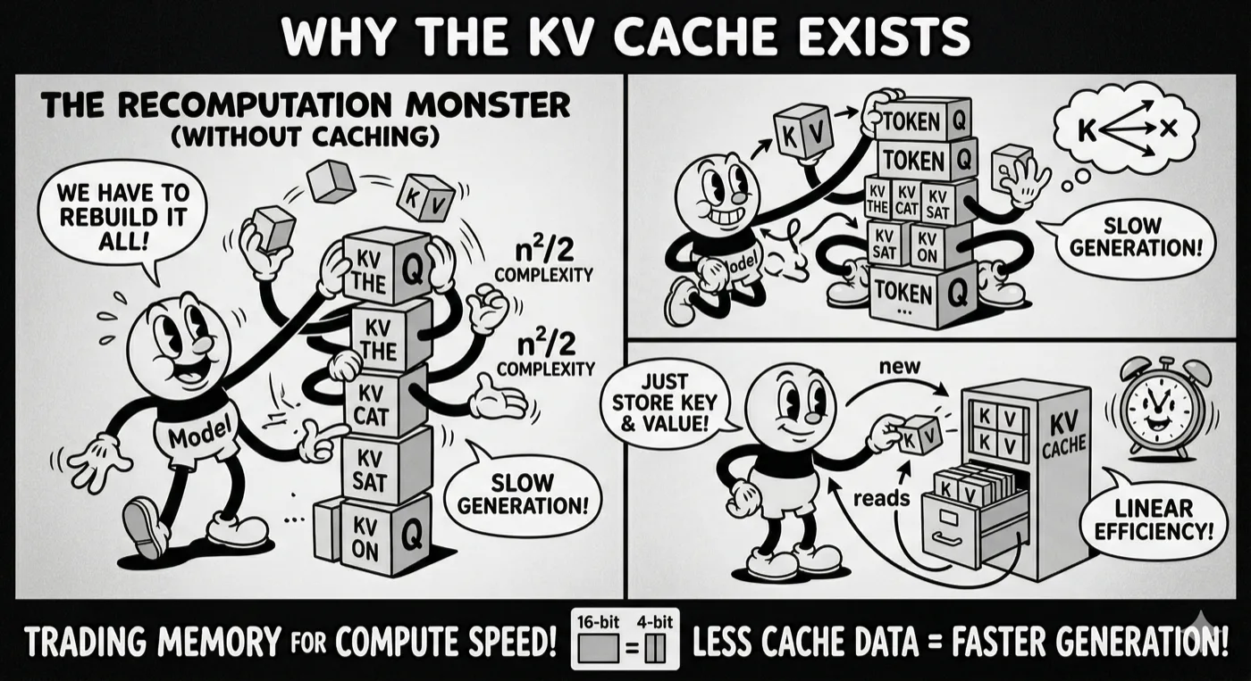
In Section 3, we established that attention requires computing dot products between the current token’s Query and the Keys of all previous tokens. Now let’s see what happens during generation without any caching.
The Recomputation Problem
Let’s generate the sentence “The cat sat on the mat” one token at a time, and watch the work pile up.
Step 1: Generate “cat”
Input: ["The"]

Work: Run "The" through all 32 layers
      - Compute Q, K, V for "The" at each layer
      - No previous tokens to attend to (first token)
      - Produce next token prediction -> "cat"

Total forward passes through the model: 1 token x 32 layers
Step 2: Generate “sat”
Input: ["The", "cat"]

Work: Run BOTH tokens through all 32 layers
      - Compute Q, K, V for "The" AGAIN (we already did this!)
      - Compute Q, K, V for "cat" at each layer
      - "cat" attends to "The" using dot products
      - Produce next token prediction -> "sat"

Total forward passes: 2 tokens x 32 layers
Step 3: Generate “on”
Input: ["The", "cat", "sat"]

Work: Run ALL THREE tokens through all 32 layers
      - Compute Q, K, V for "The" AGAIN
      - Compute Q, K, V for "cat" AGAIN
      - Compute Q, K, V for "sat" at each layer
      - Produce next token prediction -> "on"

Total forward passes: 3 tokens x 32 layers
The Pattern
Step N requires: N tokens × 32 layers = 32N operations
Total work for T tokens: 32 × (1 + 2 + 3 + ... + T) = 16T² operations

For T = 1000:  16 million forward operations
For T = 10000: 1.6 billion forward operations
This is O(T²) computation – quadratic in the number of tokens. Without caching, generating long sequences is prohibitively slow.
The KV Cache Solution
The key observation: Keys and Values for past tokens never change.
Once you’ve computed K and V for token “The” at layer 5, those values are determined. “The” is not going to update its Key based on future context. So why recompute it?
Instead:
Step 1: Compute K and V for "The" at all layers
        → Store in KV cache

Step 2: Compute K and V for "cat" at all layers
        → Store in KV cache
        → Retrieve "The"'s K and V FROM CACHE for attention
        → No recomputation of past tokens

Step 3: Compute K and V for "sat"
        → Store in KV cache
        → Retrieve "The" and "cat" K/V FROM CACHE
        → Only compute the new token's K, Q, V
Each step now does O(T) work – reading the cache and doing attention – instead of recomputing everything from scratch. Total work drops from O(T²) to O(T).
What’s in the KV Cache
At any given generation step, the KV cache contains:
For each layer L (32 layers for Llama 8B):
  For each KV head H (8 heads for GQA Llama 3.1):
    K[L][H] = matrix of shape [T × 128]   ← all past tokens' keys
    V[L][H] = matrix of shape [T × 128]   ← all past tokens' values

Total vectors: T × 32 × 8 × 2 = 512T vectors, each 128-dimensional
This is exactly what TurboQuant compresses – every one of those 128-dimensional key and value vectors, from every token, every layer, every head.
What About PagedAttention and FlashAttention?
You may have heard of other techniques that address KV cache performance. It’s worth knowing how they relate to TurboQuant:
PagedAttention (vLLM) treats GPU memory like a virtual memory system, dividing the KV cache into fixed-size “pages” and allocating them on demand. This solves memory fragmentation – preventing wasted gaps between different users’ caches – and enables efficient batching. It does not reduce the total amount of data stored. TurboQuant and PagedAttention are fully complementary: use PagedAttention to manage allocation, use TurboQuant to shrink what’s being allocated.
FlashAttention is an I/O-aware attention algorithm that recomputes certain intermediate values on the fly instead of materializing them in HBM, saving memory bandwidth during the prefill phase. It dramatically speeds up processing the initial prompt. However, it doesn’t change the size of the KV cache that accumulates during generation. Again, complementary to TurboQuant.
The KV cache ecosystem:

  PagedAttention  → fixes HOW memory is allocated (fragmentation)
  FlashAttention  → speeds up HOW attention is computed (prefill bandwidth)
  TurboQuant      → shrinks HOW MUCH is stored (cache size and read bandwidth)

  All three together: the current state of the art.
TurboQuant addresses the one thing the others don’t: the raw size of what’s stored per token.
Prefix Caching — And Why TurboQuant Is Compatible
Production serving systems (vLLM, SGLang, TGI) implement prefix caching: when multiple requests share an identical prefix — such as a system prompt or a document passed to every user — the KV cache for that prefix is computed once and reused across requests. This can eliminate large fractions of the KV computation for high-traffic deployments.
TurboQuant is compatible with prefix caching because its rotation matrix is fixed per model load, not per request. The rotation applied to a given token at a given layer is always the same, so quantizing the prefix KV cache produces deterministic, reusable results.
Without prefix caching: each request recomputes the system prompt KV
With prefix caching:    system prompt KV computed once, reused across requests
With TurboQuant + prefix caching:
  → Prefix KV is quantized once to ~3.5 bits
  → Reused across requests in compressed form
  → 4× less memory per cached prefix, same reuse benefit
TurboQuant shrinks not just each user’s individual context, but also the shared prefix pool that prefix caching relies on.
Disaggregated Serving — KV Compression Across Nodes
An increasingly important production architecture separates prefill and decode across different nodes: one set of GPUs handles the compute-intensive prompt processing (prefill), another handles the memory-intensive token generation (decode). Between them, the KV cache must be transferred over the network.
At 128K context with a 70B model, that KV transfer can be tens of gigabytes per request — a significant latency and bandwidth cost.
Standard pipeline:
  Prefill node → [transfer N GB of KV] → Decode node

With TurboQuant:
  Prefill node → [quantize KV on-the-fly to 3.5 bits]
             → [transfer N/4 GB of compressed KV]
             → Decode node (reads directly from compressed cache)
Reducing KV transfer size 4× can halve end-to-end latency for long-context requests in disaggregated setups, without changing the compute on either node. This is an application of TurboQuant that the original paper doesn’t discuss but that the community has already started exploring.
What About State Space Models?
Mamba, RWKV, and hybrid architectures like Jamba replace some or all attention layers with recurrent state space models (SSMs) that maintain a fixed-size state instead of an ever-growing KV cache. For pure SSM models, there is no KV cache and therefore no KV compression problem.
So does this make TurboQuant irrelevant as SSMs grow in adoption?
Not quite, for two reasons:
1. SSMs currently trade long-range retrieval for throughput. Attention with a KV cache can retrieve a specific fact from 100K tokens ago with near-perfect recall. SSMs compress the past into a fixed state and tend to lose fine-grained details over long contexts. The Needle-in-a-Haystack benchmark (Section 13) is exactly the task where this gap appears. For retrieval-heavy workloads — agents, RAG, legal and medical document analysis — attention with TurboQuant compression remains the better choice.
2. Hybrid architectures still have KV cache for their attention layers. Models like Jamba, Falcon Mamba, and similar hybrids interleave attention and SSM layers. The attention layers still accumulate a KV cache — smaller than a pure-attention model, but present. TurboQuant applies to exactly those layers.
Pure SSM:    No KV cache → TurboQuant not applicable
Pure Attn:   Large KV cache → TurboQuant applies fully
Hybrid:      Partial KV cache → TurboQuant applies to attention layers
TurboQuant is relevant wherever attention is used. The question isn’t “attention vs SSM” – it’s “which workloads require the retrieval accuracy that only attention provides.”