Attention — The Heart of the Transformer
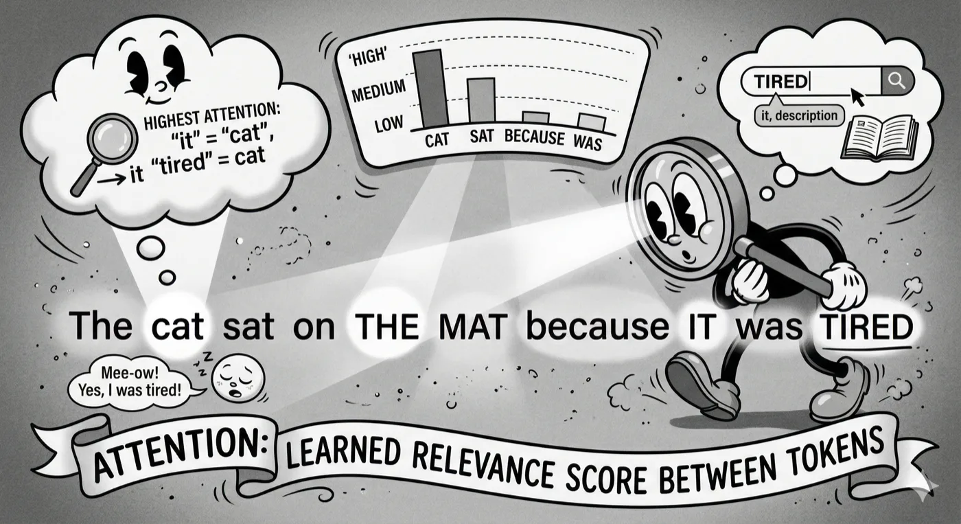
Consider this sentence:
“The cat sat on the mat because it was tired”
When the model is processing the word “tired”, it needs to figure out: what does “it” refer to? Is “it” the cat, the mat, or something else?
Attention is the mechanism that answers this question. It lets each token “look back” at all previous tokens and decide how much to care about each one.
In this example, the attention mechanism should assign:
- High attention to “cat” (because “it” = “cat”, and “tired” describes the cat)
- Medium attention to “sat” (related action)
- Low attention to “on”, “the”, “mat” (structurally present but not semantically important)
Attention = a learned relevance score between every pair of tokens.
But how does the model compute these relevance scores? That’s where Query, Key, and Value come in.
The Three Vectors: Query, Key, Value
At each layer, every token gets transformed into three separate vectors:
| Vector | Analogy | What It Represents |
|---|---|---|
| Query (Q) | A search query | “What am I looking for?” |
| Key (K) | A document title/tag | “What do I contain?” |
| Value (V) | The document content | “What information do I carry?” |
Think of it like a search engine:
- The Query is what you type into the search bar
- The Key is the title/metadata that gets matched against your query
- The Value is the actual content you get back from the matching documents
Each of these is a vector – a list of numbers. For Llama 3.1 8B, each Q, K, and V vector has 128 dimensions (per attention head).
Token "tired" at Layer 5, Head 3:
  Query: [0.23, -0.11, 0.87, ..., 0.45]    <- 128 numbers
  Key:   [-0.34, 0.56, 0.12, ..., -0.78]   <- 128 numbers
  Value: [0.67, 0.03, -0.41, ..., 0.19]    <- 128 numbers
These three vectors are produced by multiplying the token’s embedding by three different learned weight matrices – $W_Q$, $W_K$, $W_V$. These matrices are part of the model’s parameters (the billions of numbers you download).
How Attention Heads Are Shared — MHA, GQA, MQA, and MLA
In the original transformer, every attention head has its own independent Q, K, and V vectors — this is Multi-Head Attention (MHA). Every head has an independent key and value cache. This maximizes expressivity but produces the largest KV cache.
Modern models use variants that reduce the KV cache either by sharing heads across queries, or by architectural rethinking:
| Architecture | KV heads | Used by | KV Cache vs MHA |
|---|---|---|---|
| MHA (Multi-Head Attention) | 32 (one per Q head) | GPT-2, early BERT | 1× (baseline) |
| GQA (Grouped Query Attention) | 8 (shared across groups of 4) | Llama 3, Mistral, Gemma | 0.25× |
| MQA (Multi-Query Attention) | 1 (shared across all Q heads) | Falcon, PaLM | 0.03× |
| MLA (Multi-head Latent Attention) | Low-rank projection | DeepSeek-V2/V3/R1 | ~0.06–0.13×* |
GQA is now the dominant approach. Llama 3, Mistral, Gemma, and Qwen all use it. Instead of 32 independent K/V heads, GQA has 8 K/V heads each shared by 4 Q heads. This gives 4× KV cache reduction with minimal quality loss.
MLA (used by DeepSeek) is not a minor variant — it is the architectural alternative to TurboQuant. Rather than sharing heads, MLA compresses Keys and Values into a low-rank latent vector during training, and decompresses at attention time. The actual cache reduction depends on the chosen rank and head dimension — the ~0.06–0.13× figure covers known DeepSeek configurations, not a fixed ratio.
The strategic distinction matters:
GQA + TurboQuant:  Inference-time compression of a GQA cache.
                   Applies to already-trained models. No training changes needed.
                   Lossy, but bounded by theory.

MLA:               Architecture-level compression baked in at training time.
                   Requires training the model differently from scratch.
                   Achieves even smaller cache sizes, with no quantization loss.
These are not competing approaches to the same problem — they represent a choice made at different stages. If you are training a new model from scratch, MLA avoids the KV cache problem architecturally. If you are serving an already-trained GQA model, TurboQuant is the path to compression. Most open models deployed today use GQA, which is why TurboQuant is immediately applicable to the existing model ecosystem.
GQA + TurboQuant together give roughly 16× reduction versus a full-precision MHA baseline — though the exact number depends on both the GQA configuration and the TurboQuant bit-width chosen.
The Dot Product: Measuring Relevance
To compute how relevant token A is to token B, the model takes the dot product of A’s Query with B’s Key.
What Is a Dot Product?
The dot product of two vectors is simply “multiply corresponding elements, then sum.”
Query of "tired":  [0.2,  0.5, -0.3, 0.8]
Key of "cat":      [0.7,  0.4,  0.1, 0.6]
                    -----------------------
Dot product:       (0.2*0.7) + (0.5*0.4) + (-0.3*0.1) + (0.8*0.6)
                 = 0.14 + 0.20 + (-0.03) + 0.48
                 = 0.79   (high → "tired" is very relevant to "cat")
Compare to the dot product of “tired” with “the”:
Query of "tired":  [0.2,  0.5, -0.3, 0.8]
Key of "the":      [0.1, -0.2,  0.0, 0.1]
                    -----------------------
Dot product:       (0.2*0.1) + (0.5*-0.2) + (-0.3*0.0) + (0.8*0.1)
                 = 0.02 - 0.10 + 0 + 0.08
                 = 0.00   (low → "tired" doesn't care about "the")
High dot product = high attention = “these two tokens are relevant to each other.”
From Scores to Weights: The Softmax
The raw dot products (attention scores) get converted to probabilities via softmax:
$$\text{Attention}(q, K, V) = \text{softmax}!\left(\frac{q K^T}{\sqrt{d}}\right) V$$
Softmax takes a vector of scores and converts them to positive weights that sum to 1.
Raw scores:   [0.79, 0.23, 0.18, 0.00, 0.15, 0.05]
             → softmax →
Attention:    [0.47, 0.12, 0.11, 0.08, 0.10, 0.09]  (sums to ~1)

Token "cat" gets 47% of the attention weight.
Token "the" gets only 8-9%.
The final output for “tired” is a weighted sum of all previous tokens’ Value vectors, where the weights come from attention:
Output = 0.47 × V("cat") + 0.12 × V("sat") + 0.11 × V("on") + ...
This is the token’s updated representation – enriched with contextual information from the tokens that matter most to it.
Why Q Is Not Cached But K and V Are
Notice what happens at generation time:
- Query: Used to score “what does the current token care about?” Generated fresh for every new token.
- Key: Represents “what does each past token contain?” — computed once when the token is first processed, then cached.
- Value: Represents “what information does each past token carry?” — same, computed once and cached.
This is exactly why only K and V get cached. Queries are local to the current step; Keys and Values belong to all past context and are reused every step.
The KV cache is just the accumulated Keys and Values for every past token, across every layer, saved to avoid recomputation.
And this is precisely what TurboQuant compresses.
A Critical Implementation Detail: RoPE Rotates Keys Before Caching
One thing the simplified description above glosses over: in the majority of modern models — Llama, Mistral, Gemma, Qwen, and others — Keys are not cached in their raw form. These models use Rotary Position Embeddings (RoPE), which applies a position-dependent rotation to every Key (and Query) vector before the dot product is computed.
RoPE in a nutshell:
  Raw Key for token at position p:  k_raw   (model output, position-agnostic)
  Rotated Key:                      k = R(p) · k_raw  (what actually gets cached)

  R(p) is a rotation matrix that encodes position p.
  The same word at position 10 has a different Key than at position 100.
The important practical consequence: TurboQuant quantizes after the RoPE rotation is applied — it compresses $k = R(p) \cdot k_\text{raw}$, not the raw $k_\text{raw}$. Any correct implementation must apply RoPE first, then quantize. Implementations that quantize pre-rotation and apply RoPE at lookup time will produce subtly incorrect attention scores.
This is not a gap in TurboQuant — it quantizes whatever vector it receives — but it is a real correctness footgun for anyone building from scratch.